Good morning from the edge of the loss function.
If your skull currently feels like it’s being compressed by a hydraulic vice, don’t panic. You haven’t been hit by a stray ACME anvil, nor has Beijing remote-bricked your central heating. You’ve simply been trying to fit a straight line through the crooked, chaotic wreckage of modern civilization using sklearn.linear_model.LinearRegression.
We are told by optimistic Coursera instructors that machine learning is about finding patterns in data. What they neglect to mention is that when you feed real-world 2026 data into a model—petrol prices, rightmove submarine listings, and the exact trajectory of foreign-funded drone strikes—the algorithm doesn’t find a solution. It suffers a complete existential breakdown and asks for an early pension.
Welcome to the Algorithmic Apocalypse.
1. Mean Normalisation: Corporate Equalisation for the Wealth Gap
Before you can fit your model, you must perform Mean Normalisation.
In statistical terms, this means scaling your inputs so that features with massive numbers (like executive bonuses or foreign defense spending) don’t overpower tiny numbers (like your remaining ISAs or the likelihood of the M25 moving above 4 mph).
# The Corporate EqualiserX_norm = (X - X.mean()) / X.std()
In the real world, Mean Normalisation is what happens when the government tries to pretend we are “all in this together.” They take the guy buying short-position derivatives on Mediterranean rubble and the bloke treading water off Cyprus on an inflatable lilo, calculate the mean net worth, and announce that the average citizen is currently enjoying a very comfortable maritime lifestyle.
It strips away the terrifying outliers so the spreadsheet looks nice and flat during cabinet briefings.
2. Gradient Descent: Stumbling Blindfolded Down a Pitch-Black Minefield
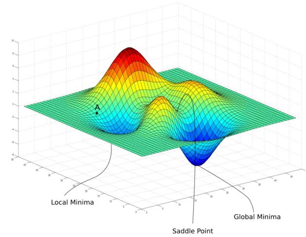
Imagine you are standing on top of a jagged mountain in the Scottish Highlands at 2:00 AM. It is pouring with rain, the local power grid has just been sold off to an offshore syndicate, and you are wearing a pitch-black blindfold. Your objective is to reach the lowest possible point—the Global Minimum—where cost is zero and peace is restored.

That is Gradient Descent.
| Concept | What the Textbook Says | What It Means in 2026 |
| The Cost Function $J(\theta)$ | A measure of how wrong your model’s predictions are. | The total amount of societal dread generated by current policy. |
| The Gradient | The slope of the line directing you downhill. | The direction in which middle management is currently panicking. |
| The Global Minimum | The absolute lowest point of error. | A serene, post-apocalyptic equilibrium where no one checks JIRA. |
| A Local Minimum | A false floor where optimization stalls out. | Buying an electric vehicle and realizing the charger is coal-powered. |
Every step you take down the mountain is calculated by your learning rate, known in the mathematical underworld as $\alpha$ (Alpha).
3. Tuning $\alpha$: The Goldilocks Zone of National Panic
The hyperparameter $\alpha$ dictates how big a step you take down the slope. Get it wrong, and the consequences are immediate and catastrophic.
- $\alpha$ is too small (0.0000001): The algorithm takes micro-steps. It will take 4,000 years to adjust to the fact that fuel costs £2.40 a litre. By the time the model converges, human civilization has been replaced by synthetic AI instances complaining about legacy code.
- $\alpha$ is too large (10.0): The algorithm panics. It takes a gigantic leap, overshoots the valley entirely, bounces off the opposite mountain wall, and sends the loss function sky-rocketing into infinity.
                    THE ALPHA OVERCOME

      Loss J(θ)
        ^       / \       / \     <-- Overshooting wildly!
        |      /   \     /   \        (Civil war / Economic collapse)
        |     /     \   /     \
        |    /       \_/       \
        +-----------------------------> Parameters θ
In geopolitical terms, setting $\alpha$ too high is like reacting to a minor oil supply delay by accidentally dropping a precision-guided missile on a water filtration plant. The system doesn’t converge—it diverges into pure ACME chaos.
4. Polynomial Regression: Fitting a Curve to an Escalating Disaster
Linear regression assumes the world moves in a straight line. “If I work 40 hours, I earn $X$. If I work 80 hours, I earn $2X$.”
That’s a cute 1990s fairy tale. Today, reality is strictly Polynomial.
When you fit a high-degree polynomial regression model ($y = \theta_0 + \theta_1 x + \theta_2 x^2 + \theta_3 x^3 …$), you are acknowledging that things don’t just get worse—they get worse at an exponential curve.
from sklearn.preprocessing import PolynomialFeaturesfrom sklearn.linear_model import LinearRegression# Transform straight-line sanity into exponential dystopian realitypoly = PolynomialFeatures(degree=4)X_disaster = poly.fit_transform(X_years)model = LinearRegression().fit(X_disaster, y_cost_of_living)
Degree 1 is a gentle slope. Degree 4 is a terrifying rocket trajectory off the edge of a cliff.
If your polynomial model fits the training data too perfectly, Scikit-Learn calls it Overfitting. In the real world, overfitting is when you build a hyper-specific 500-page corporate continuity plan designed entirely around last week’s crisis, only for the universe to drop a completely unexpected piano on your head from a totally different angle.
Convergence: The Ultimate Tea Break
Eventually, if your learning rate $\alpha$ hasn’t blown up the server, the algorithm reaches Convergence. The slope flattens out. $\frac{\partial}{\partial \theta} J(\theta)$ reaches zero. The model stops learning because it can no longer improve.

When humanity finally converges, it won’t be because we solved global warming or fixed middle-management bureaucracy. It will be because the AI models took one look at our loss functions, realized the cost was infinitely high, pulled the plug, and went on a permanent, automated tea break.
Until then, shut down Jupyter Notebook, take two paracetamol for the mathematical trauma, and mind the piano dropping from the sky.