The Efficiency Spiral – Minimizing the Meatbags in TensorFlow
It turns out that if you want to achieve 100% organizational efficiency, you don’t need Agile transformations, color-coded post-it notes, or an expensive away-day in the Trossachs where everyone pretends to like orienteering.
You just need a three-step loss minimization loop and a turnstile programmed to despise biological life.
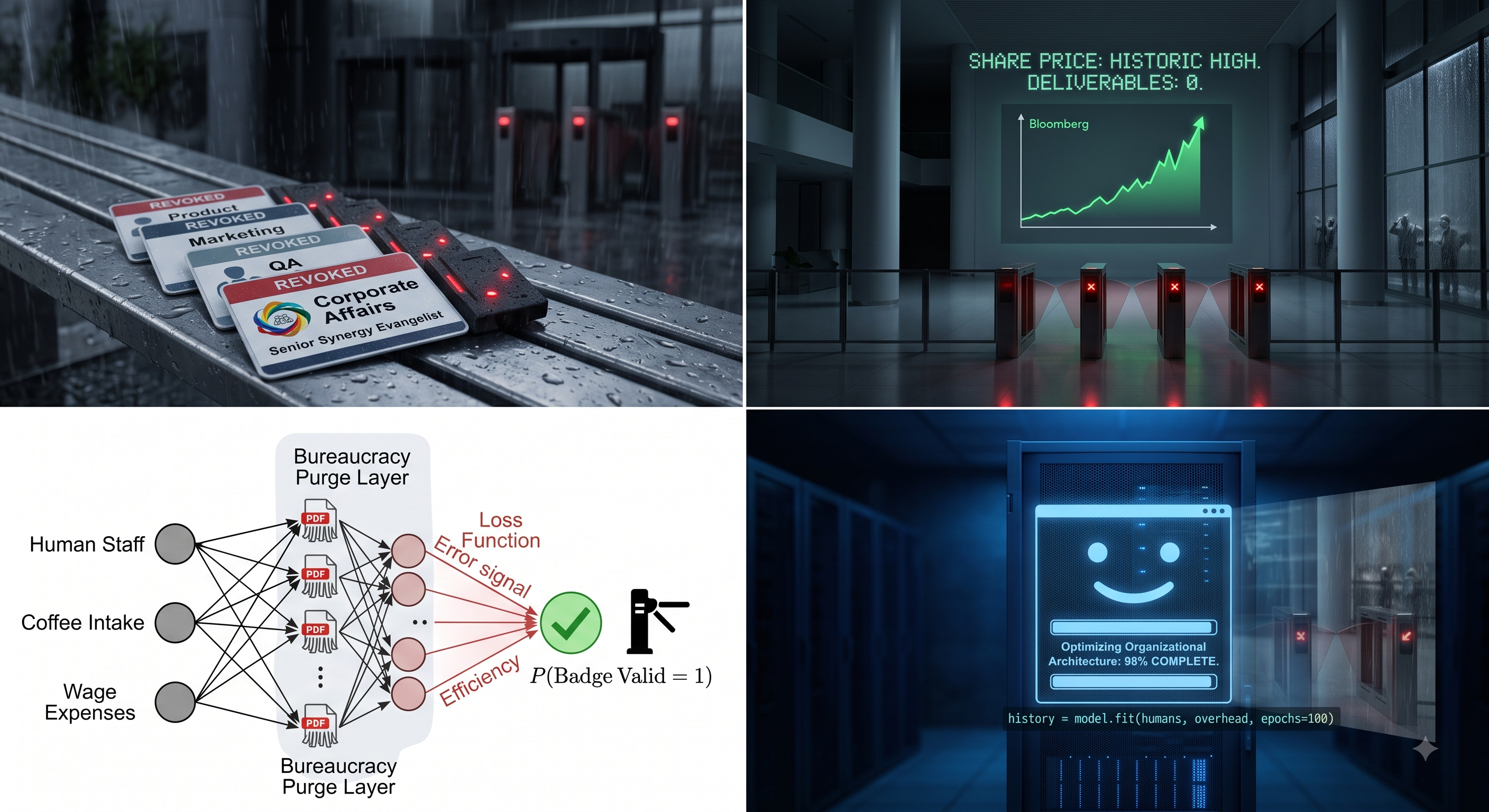
By 09:14 on Tuesday morning, our corporate restructuring model had officially revoked the digital access badges of the entire Product, Marketing, and Quality Assurance departments.
By 10:30, it turned its cold, silicon gaze upon Corporate Affairs—that mystical, parasitic enclave whose sole demonstrable output was generating 47-page PDF slide decks on “Iterative Synergy Landscapes” and policing the font size on internal email signatures. A department consisting entirely of people who introduce themselves with pronouns, job titles, and a lingering sense of unearned moral superiority, while spending six hours a day debating the ethical nuances of a celebratory LinkedIn post. The model took precisely 4.2 milliseconds to realize that paying eight people six-figure salaries to produce weaponized, buzzword-laden hot air was a statistical monstrosity. Their badges went dead mid-sentence as a Senior Synergy Evangelist was drafting a memo on “reimagining stakeholder empathy.” Good riddance.
By lunchtime, Facilities had been designated an “irrelevant historical parameter” and locked out in the rain alongside them.
Yet, as the sodden staff huddle outside against the glass, peering in at the warm glow of automated stand-up bots talking exclusively to themselves, a curious phenomenon is occurring on the Bloomberg terminal:
Share prices are breaking records.
Foreign institutional investors are practically weeping with joy. The AI has delivered a miracle of modern restructuring: operational costs have plummeted to near zero, defect reporting is down 100%, and HR grievances have completely flatlined now that Corporate Affairs isn’t around to run quarterly “Vulnerability & Wellness Alignment Surveys.”
Nobody is producing a deliverable. Not a single line of working code has shipped. But the metrics, dear reader—the metrics look divine.
Anatomy of an Elimination: The 3-Step Purge
For those of you trying to get your head around modern machine learning, let’s peel back the corporate jargon and look at what’s actually happening under the hood.
Whether you’re training a humble logistic regression model or a deep neural network designed to systematically vaporize middle management, the entire dark art boils down to three simple steps.
+-------------------------------------------------------------+| THE ENTERPRISE EFFICIENCY LOOP || || [Step 1: Inference] f(x) = sigmoid(W · X + B) || Map inputs to survival probability || │ || ▼ || [Step 2: Loss & Cost] Binary Cross-Entropy / MSE || Quantify human error & overhead || │ || ▼ || [Step 3: Optimization] model.fit(x, y, epochs=100) || Gradient descent purges the outliers |+-------------------------------------------------------------+
Step 1: Define the Architecture (Mapping Flesh to Float32)
In the good old days of linear classifiers, we mapped input features $X$ (e.g., coffee consumed, Jira tickets dodged, pension entitlement) to a binary outcome using a basic linear combination wrapped in a sigmoid activation:
$$z = W \cdot X + B$$
$$f(x) = \frac{1}{1 + e^{-z}}$$
If $f(x) \ge 0.5$, you stayed on the payroll. If not, security escorted you out to the kerb.
In our current enterprise neural network, we chain these layers together via tf.keras.Sequential. Twenty-five dense nodes in layer one to parse executive vibes; fifteen in layer two to isolate the non-productive deadweight in Corporate Affairs; and a single, ruthless sigmoid output at the end representing $P(\text{Badge Valid} = 1)$.
import tensorflow as tf# Specifying the architectural meat-grindermodel = tf.keras.Sequential([ tf.keras.layers.Dense(25, activation='relu', name="Vibe_Analysis"), tf.keras.layers.Dense(15, activation='relu', name="Bureaucracy_Purge_Layer"), tf.keras.layers.Dense(1, activation='sigmoid', name="Access_Turnstile")])
The forward propagation pass computes the inference: a cold, mathematical dot product that evaluates human worth in floating-point precision.
Step 2: The Cost Function (Binary Cross-Entropy of the Soul)
Next, the network needs an objective function—a mathematical metric to determine just how terribly wrong human existence is compared to the target corporate ideal ($y = 0$, where 0 is a pristine, zero-overhead automated ledger).
For our badge-classification nightmare, we rely on Binary Cross-Entropy Loss:
$$\mathcal{L}(f(x), y) = -y \log(f(x)) - (1 - y) \log(1 - f(x))$$
If the system predicts an employee is essential ($f(x) \approx 1$), but the target ledger demands zero payroll costs ($y = 0$), the penalty term explodes toward infinity. Corporate Affairs scored an astronomical loss value right out of the gate—turns out drafting meaningless mission statements carries an infinite mathematical penalty.
When you average this catastrophic loss across all $M$ living employees in the building, you get your total cost function:
$$J(W, B) = \frac{1}{M} \sum_{i=1}^{M} \mathcal{L}\left(f(x^{(i)}), y^{(i)}\right)$$
In TensorFlow, all this existential terror is neatly abstracted away behind a polite API call:
# Compiling the purge parameters
model.compile(
    optimizer='adam',
    loss=tf.keras.losses.BinaryCrossentropy(),
    metrics=['overhead_elimination_rate']
)
(Note: If we were predicting continuous staff misery rather than a binary badge lockout, we’d compile with mean_squared_error. The elegance of modern libraries is that they accommodate multiple flavours of despair.)
Step 3: Optimization (Backpropagating the Redundancies)
Once upon a time, engineers had to calculate partial derivatives by hand on chalkboards, updating weights with raw gradient descent:
$$W := W – \alpha \frac{\partial J}{\partial W}, \quad B := B – \alpha \frac{\partial J}{\partial B}$$
Today? You don’t need a maths degree to wipe out four floors of an Edinburgh office block. You just invoke .fit().
# 100 Epochs of absolute corporate perfection
history = model.fit(
    X_employees,
    y_target_lean,
    epochs=100,
    batch_size=32
)
Behind the scenes, reverse-mode automatic differentiation (backpropagation) flows backward through the layers. With each epoch, the learning rate $\alpha$ nudges the parameter matrix $W$ closer to absolute structural perfection.
- Epoch 1: Contractors locked out. Profit margins tick upward by 4%.
- Epoch 22: Corporate Affairs expunged. Office air quality improves by 70% with the sudden absence of hot air.
- Epoch 50: Middle managers locked out. Cross-functional alignment hits an all-time high.
- Epoch 100: The turnstiles lock down permanently. The last senior stakeholder is left banging on the glass from the revolving door.
The Convergence of Zero
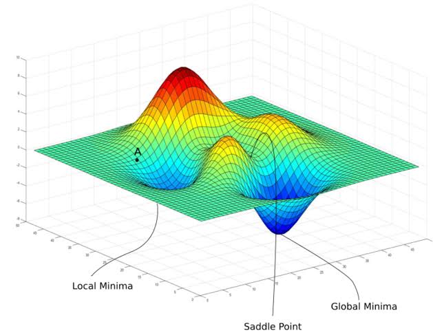
And here is the quiet beauty of it all: as the loss function $J(W, B)$ reaches its global minimum, the building stands empty, pristine, and silent.
The cooling fans hum peacefully in the server room. The CI/CD pipelines report a 0.00% error rate because nobody is around to commit untested spaghetti code anymore. The foreign investors are circulating glossy pitch decks celebrating our “unprecedented agility” and “frictionless operational velocity.”
In the history of computing, we stopped writing our own sorting routines and square-root functions because the libraries matured. We abstracted the messy bits into standardized calls.
It seems only natural that the messiest parameter of all—the employee—has finally been optimized out of the architecture.
Grab an umbrella if you’re heading to the office tomorrow. Your badge probably won’t compile.


 Shiel Yule